Graph Convolutional Networks for Temporal Vulnerability Classification in Obstetric Hospitalization Flows from SUS
Tiago Mota de Oliveira, Claudemir Casa
- Published in
- SIBGRAPI 2026 — 38th Conference on Graphics, Patterns and Images, Goiânia, Brazil
A health region is a network — so why not model it as one?
When a pregnant woman in a small municipality needs hospital care, she often does not get it where she lives. She travels. Across Brazil's Unified Health System (SUS), specialised obstetric infrastructure concentrates in regional hubs, and the surrounding municipalities refer their patients inward. The result is a genuine network: municipalities are not independent data points, they are nodes connected by recurrent referral flows.
Most analyses of these flows nonetheless flatten them into a table — origin-destination counts per municipality, one row each, topology discarded. Graph Neural Networks exist precisely to avoid that, and they have worked well on traffic, mobility, and epidemic forecasting. So we asked a direct question:
If we build the referral network explicitly and feed it to a Graph Convolutional Network (GCN), does the topology buy us anything?
The honest answer we found is no — and the more interesting contribution of this paper is the controlled experiment that says why not, and shows the cause is a correctable modelling choice rather than a verdict on graph learning.
- obstetric hospitalizations analysed (2025)
- 35,022
- municipalities in the 2nd Health Region of Paraná
- 29
- random seeds behind every reported number
- 30
The data
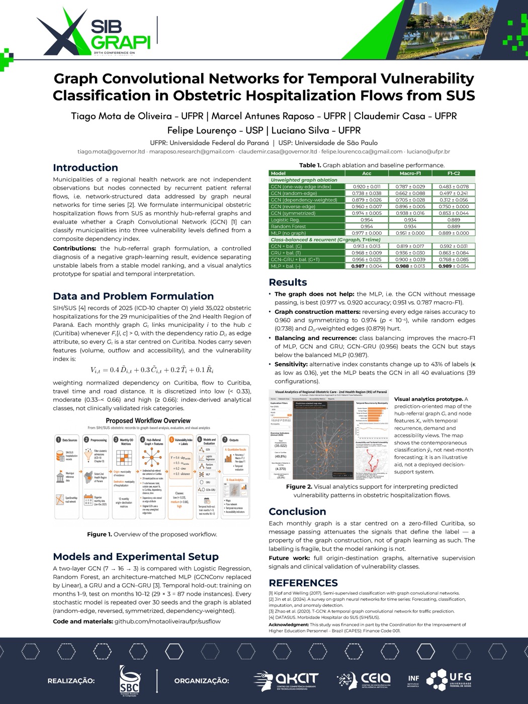
Hospitalization records came from the public SIH/SUS dataset for all twelve months of 2025. Each record carries the municipality of residence, the municipality of hospitalization, the primary diagnosis (ICD-10), and the competence month.
We kept the obstetric cases — ICD-10 chapter O, covering pregnancy, childbirth and the puerperium — and restricted both residence and hospitalization to the 29 municipalities of the 2nd Health Region of Paraná, whose hub is Curitiba. That yields 35,022 hospitalizations across twelve months.
Turning a year of flows into twelve graphs
For each month we computed a flow matrix and built one graph over the same fixed set of 29 municipalities. A municipality is linked to Curitiba whenever at least one of its residents was hospitalised there that month, and the edge carries that municipality's dependency ratio on the hub.
Two structural properties of this construction turn out to decide everything that follows:
- Every edge touches Curitiba, so each monthly graph is a star — there are no municipality-to-municipality edges, and the 5–9 municipalities with no flow to the hub in a given month are isolated.
- The edge attribute is also a node feature and the dominant term of the label, so it is not independent of the supervision signal.
Each node carries seven features, grouped into three families:
| Family | Features | What it captures |
|---|---|---|
| Volume | total | Local obstetric demand — the denominator every rate normalises against |
| Outflow | ext, export_pct, to_curitiba, curitiba_dep | How much care leaves the municipality, and where it goes |
| Accessibility | distance_km, time_min | The cost of that displacement by road |
Distance and travel time are both kept despite being correlated, because terrain and road quality make them diverge. No feature was dropped by selection, so no supervised choice was made on the data used for evaluation.
The label: a composite vulnerability index
Supervision comes from a composite index combining four normalised features — dependency on Curitiba (weight 0.4), flow to Curitiba (0.3), travel time (0.2) and road distance (0.1) — discretised into three equal-width bands:
| Class | Index range | Reading |
|---|---|---|
| 0 | below 0.33 | Low vulnerability |
| 1 | 0.33 – 0.66 | Moderate vulnerability |
| 2 | 0.66 and above | High vulnerability |
The weights were fixed a priori by domain reasoning, not fitted to data. These are index-derived analytical classes, not clinically validated risk categories — a distinction we return to below, and one the sensitivity analysis takes seriously.
Top tip
Note what this means for the learning problem: the label is a thresholded linear function of four of the seven inputs. Any model that can recover that combination should do well. That property is not a flaw in the experiment — it is the lens through which every result has to be read.
The experiment
The twelve monthly graphs were split temporally: train on months 1–9, test on months 10–12. Each graph contributes 29 node-level instances, so the test set holds 87. No model is retrained on the test months.
Against a two-layer GCN (7 → 16 → 3) we ran five comparisons:
- Logistic Regression and Random Forest — classic tabular baselines on the same seven features.
- MLP — identical to the GCN in width, activation, optimiser and schedule, with the graph convolution replaced by a linear layer. This is the controlled counterfactual: any gap between GCN and MLP is attributable to message passing, not to capacity.
- GRU and GCN–GRU — recurrent models that carry per-node state across months, to test whether the temporal dimension holds signal the snapshot models miss.
Every stochastic model was retrained over 30 seeds, and the graph itself was ablated four ways: random edges, reversed edges, symmetrised edges, and edges weighted by the dependency ratio.
What the numbers said
| Model | Accuracy | Macro-F1 | F1 (class 2) |
|---|---|---|---|
| GCN (as stored) | 0.920 ± 0.011 | 0.787 ± 0.029 | 0.483 ± 0.078 |
| GCN (random edges) | 0.738 ± 0.038 | 0.662 ± 0.088 | 0.497 ± 0.241 |
| GCN (dependency-weighted) | 0.879 ± 0.026 | 0.705 ± 0.028 | 0.312 ± 0.056 |
| GCN (reversed edges) | 0.960 ± 0.007 | 0.896 ± 0.005 | 0.750 ± 0.000 |
| GCN (symmetrised) | 0.974 ± 0.005 | 0.938 ± 0.016 | 0.853 ± 0.044 |
| Logistic Regression | 0.954 | 0.934 | 0.889 |
| Random Forest | 0.954 | 0.934 | 0.889 |
| MLP (no graph) | 0.977 ± 0.000 | 0.951 ± 0.000 | 0.889 ± 0.000 |
And with class balancing and the recurrent models, on the same test set:
| Model | Uses | Accuracy | Macro-F1 | F1 (class 2) |
|---|---|---|---|---|
| GCN + balanced | graph | 0.913 ± 0.013 | 0.819 ± 0.017 | 0.592 ± 0.031 |
| GRU + balanced | time | 0.968 ± 0.009 | 0.936 ± 0.030 | 0.863 ± 0.084 |
| GCN–GRU + balanced | graph + time | 0.956 ± 0.025 | 0.900 ± 0.039 | 0.768 ± 0.085 |
| MLP + balanced | neither | 0.987 ± 0.004 | 0.988 ± 0.013 | 0.989 ± 0.034 |
Four findings follow.
The graph does not help. The MLP differs from the GCN only by the removal of message passing, and it wins on every metric — 0.977 against 0.920 accuracy, 0.951 against 0.787 macro-F1. On this graph, message passing is a measurable loss, not a tie.
Edge orientation is an artifact — and a revealing one. Reversing every edge raises accuracy to 0.960; symmetrising raises it to 0.974 (both p < 10⁻⁴ on a paired t-test across seeds). Since the stored orientation is arbitrary, this is the smoking gun: in the original configuration, message passing pushed Curitiba's feature vector onto the leaves — and Curitiba, which never appears as a residence origin in the filtered data, is zero-filled in all twelve months. The hub was broadcasting nothing, and diluting each municipality's own signal in the process. Reverse the edges and every leaf keeps its own features through the self-loop.
The real network still beats a random one. A random-edge control with the same node and edge counts collapses to 0.738, well below the observed star's 0.920. The topology is not noise — it just is not the structure that determines this label.
Weighting edges by dependency makes it worse (0.879), despite dependency being the dominant term of the label. It amplifies the same dilution.
Recurrence tells a consistent story: GCN–GRU improves on the plain GCN (+0.043 balanced, p < 10⁻⁴) but still loses to the graph-free MLP, and the GRU alone underperforms the MLP. There is no recoverable temporal signal beyond each month's own features.
Are the labels themselves trustworthy?
A fair objection to any index-based target: change the constants, change the conclusion. We tested that directly, rebuilding the labels under six named weight vectors, 30 symmetric-Dirichlet draws, and four threshold pairs.
The result splits cleanly in two:
- The labelling is fragile. Alternative constants move up to 43% of labels (Cohen's κ as low as 0.16), and the high-vulnerability class ranges from 0 to 37 test instances against 5 under the published constants. The three classes are an analytical convention, not a stable partition of these municipalities.
- The model ranking is not. The no-graph MLP beats the GCN in all 40 evaluations, spanning 39 distinct configurations.
So the negative result is about the graph, not about the particular constants we happened to choose. That separation — fragile labels, stable conclusion — is one of the things we most wanted this paper to establish.
Why the graph lost, in one sentence
Each monthly graph is a star centred on a zero-filled hub, so message passing attenuates exactly the signals the label thresholds. That is a property of the graph construction, not of graph learning as such — and it points at a concrete fix: encode the full origin-destination structure instead of only the hub column, and impute Curitiba's features from its role as a destination rather than zero-filling them.
The visual analytics prototype
Alongside the models we built a short prototype that puts the monthly referral graph on a map, next to temporal recurrence, demand, and accessibility views. It shows the contemporaneous classification, not a next-month forecast, and it is an illustrative analytical aid — not a deployed, user-evaluated decision-support system.
Limitations we want stated plainly
- Target by construction. The labels are a thresholded linear function of four of the seven inputs, which favours any model that can recover that combination. A target external to the features — clinical outcomes, maternal morbidity, future flow volumes — is needed before this benchmark can test what a graph model is really capable of.
- Graph construction. The monthly graphs keep only municipality-to-hub links. The negative result is evidence about this graph, not about graph-based referral formulations in general.
- Normalisation scope. Feature scaling is fitted per month, which avoids cross-month leakage but means the protocol is temporally separated at model fitting, not at preprocessing.
- Small minority class. Class 2 holds only 5 test instances (5.7%), and its F1 varies with a standard deviation of up to 0.241 across seeds — so our conclusions rest on accuracy, which is far more stable.
- Data lag. SIH/SUS records face administrative processing delays, so this is a framework for retrospective analysis and planning, not real-time monitoring.
- Applicability. This is analytical support for flagging persistent dependency and characterising regional centralisation — not a directive for clinical or administrative decisions. Operational use would require validation with health managers and clinicians, which we did not carry out.
At SIBGRAPI 2026
The work was presented at SIBGRAPI 2026, the 38th Conference on Graphics, Patterns and Images, in Goiânia.



Code and materials
The implementation, the monthly graph builders, and the ablation, temporal and sensitivity scripts are published at github.com/motaoliveiraufpr/susflow.
This paper continues the group's line of work on turning real-world signals into structured, analysable data — see also our smartwatch-based system for driver stress and the multimodal emotion-recognition battery for children.
Acknowledgments
This study was financed in part by the Coordination for the Improvement of Higher Education Personnel — Brazil (CAPES), Finance Code 001.
How to cite
de Oliveira, T. M., Raposo, M. A., Casa, C., Lourenço, F. and Silva, L. (2026). Graph Convolutional Networks for Temporal Vulnerability Classification in Obstetric Hospitalization Flows from SUS. In Proceedings of the 38th Conference on Graphics, Patterns and Images (SIBGRAPI 2026), Goiânia, Brazil.
This is a plain-language adaptation of the paper, prepared for a general audience. For the full formulation, figures, statistical tests and complete reference list, please consult the poster or the code repository.